Simply supported beam subjected to vehicular live load

1

Structural model

Consider a simply supported beam of span \(L\), with a fixed section \(S_x\) at \(0 \lt x \lt L\). A vehicle is represented by downward axle loads \(P_i\), whose fixed offsets \(d_i\) are measured from a reference axle at position \(s\). Moving the vehicle changes every axle position by the same amount; axle spacings must remain fixed.

\[ f_I(z)=0\quad\text{for }z<0\text{ or }z>L,\qquad z_1(s)=s,\qquad z_{i+1}(s)=z_i(s)+d_{i,i+1}. \]

\[ L=z_A+L_q+z_B,\qquad a_j=z_A,\qquad b_j=z_A+L_q. \]

Distributed loads \(q_j(z,s)\) act over prescribed intervals. Only axles on the span and the portions of those intervals intersecting the span contribute. An empty intersection contributes zero. A distributed load may move with the vehicle or occupy a separately prescribed lane region; the loading rule determines its position, not the influence line. Overlapping patches add unless the load model explicitly excludes that overlap.

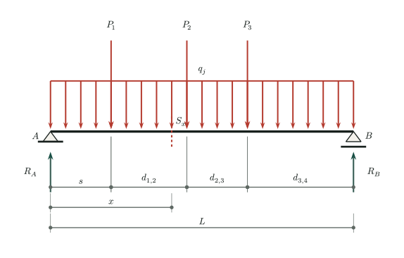
General load model: axle loads P_i, distributed load q_j, reference position s, successive axle spacings, and section position x.

Downward loads are positive inputs and upward support reactions are positive outputs. Positive shear acts downward on the cut face of the left free body; positive bending moment is sagging (tension in the lower fibers). Linear, small-displacement behavior is assumed.

2

Superposition and signed areas

For any response \(E\), let \(\eta_E(z)\) be its influence-line ordinate due to a downward unit load at \(z\). At a given vehicle position, multiply each axle load by its own ordinate and integrate each distributed load against the same influence line. Add all contributions algebraically.

\[ \boxed{F(s)=\sum_i P_i\,f_I(z_i(s)) +\sum_j\int_{a_j}^{b_j}q_j(z,s)\,f_I(z)\,dz.} \]

For a constant intensity \(q\) on a clipped interval \([a,b]\), its effect is \(q\) times the signed area under the influence line. On a straight branch this area is exactly a trapezoid. Reaction and shear ordinates are dimensionless, so their areas have units of m; moment ordinates have units of m, so their areas have units of m².

\[ F_{qj}=q_j A_{Ij},\qquad A_{Ij}=\int_{a_j}^{b_j}f_I(x)\,dx,\qquad A_{Ij}=\frac{b_j-a_j}{2}\bigl[f_I(a_j)+f_I(b_j)\bigr] \quad\text{on a straight branch.} \]

Split the interval at every change of slope or jump, especially at \(z=x\). For shear, keep the negative and positive areas with their signs and use the appropriate one-sided ordinate at each end of a branch. Do not apply one trapezoid across the shear jump or moment peak. For nonuniform intensity, use the integral rather than a constant \(q\) times area.

Review the derivation of the unit-load influence lines

3

Support reactions

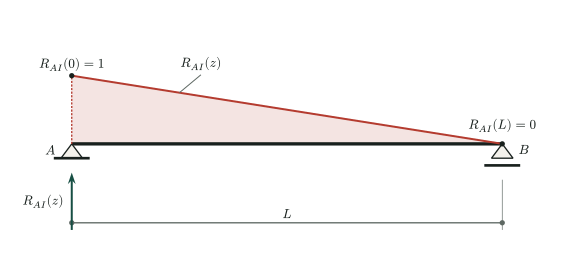
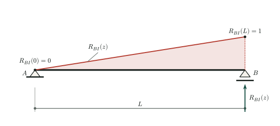
The support-reaction influence lines are linear throughout the span. Apply superposition with the following ordinates:

\[ f_{R_A}(z)=\frac{L-z}{L},\qquad f_{R_B}(z)=\frac{z}{L}. \]

\[ \begin{aligned} R_A(s)&=\sum_i P_i f_{R_A}(z_i(s)) +\sum_j\int_{a_j}^{b_j}q_j(z,s)f_{R_A}(z)\,dz,\\ R_B(s)&=\sum_i P_i f_{R_B}(z_i(s)) +\sum_j\int_{a_j}^{b_j}q_j(z,s)f_{R_B}(z)\,dz. \end{aligned} \]

For a uniform patch on \([a,b]\), the same result follows by placing its resultant \(q(b-a)\) at its centroid \((a+b)/2\). This substitution also works for moment only if the entire patch lies on one straight branch of the moment influence line; it generally fails for a patch crossing the section.

\[ R_{A,q}=q_j A_{R_Aj},\qquad R_{B,q}=q_j A_{R_Bj}, \qquad F_{qj}=q_jL_q. \]

Influence line of right support reaction

4

Shear force

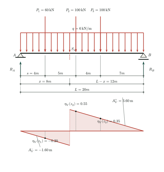
Keep the section fixed and vary the load coordinate \(z\). Axles to the left of the section contribute negative shear ordinates; axles to the right contribute positive ordinates.

\[ f_V(z)= \begin{cases} -z/L,&0\le z\lt x,\\ (L-z)/L,&x\lt z\le L. \end{cases} \qquad f_V(x^-)=-\frac{x}{L},\quad f_V(x^+)=\frac{L-x}{L}. \]

\[ \boxed{V_x(s)=\sum_iP_i\,f_V(z_i(s)) +\sum_j\int_{a_j}^{b_j}q_j(z,s)\,f_V(z)\,dz.} \]

If an axle lies exactly at the section, report the two one-sided shear values instead of averaging the ordinates. The influence-line jump is +1 as the axle moves from left to right, so the response jump is +\(P_i\). The value at a single point does not affect a distributed-load integral.

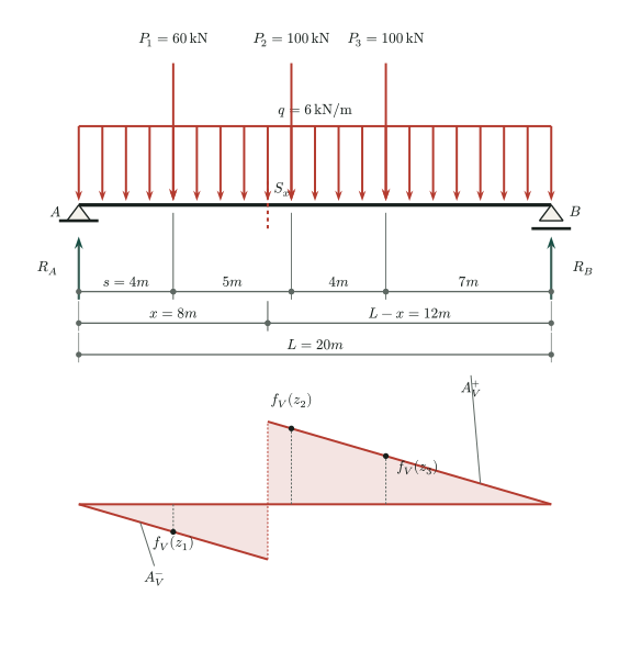
General shear influence-line construction with signed areas and ordinates at the axle positions.

For the full-span uniform load shown, the two triangular areas give:

\[ A_V^-=-\frac{x^2}{2L},\qquad A_V^+=\frac{(L-x)^2}{2L}, \qquad V_{x,q}=q(A_V^-+A_V^+)=q\left(\frac L2-x\right). \]

5

Bending moment

The bending-moment influence line is continuous and triangular, with positive ordinates for downward loads anywhere inside the span. Its peak occurs at the fixed section.

\[ f_M(z)= \begin{cases} z(L-x)/L,&0\le z\le x,\\ x(L-z)/L,&x\le z\le L. \end{cases} \qquad f_M(x)=\frac{x(L-x)}{L}. \]

\[ \boxed{M_x(s)=\sum_iP_i\,f_M(z_i(s)) +\sum_j\int_{a_j}^{b_j}q_j(z,s)\,f_M(z)\,dz.} \]

General bending-moment influence-line construction with ordinates at the axle positions.

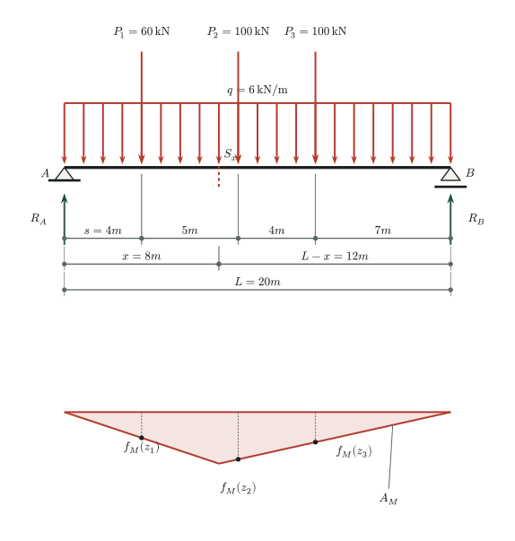
For a uniform load over the full span, the area of the complete triangle gives:

\[ A_M=\frac12L\,\frac{x(L-x)}{L}=\frac{x(L-x)}2,\qquad M_{x,q}=qA_M. \]

6

Worked example at one position

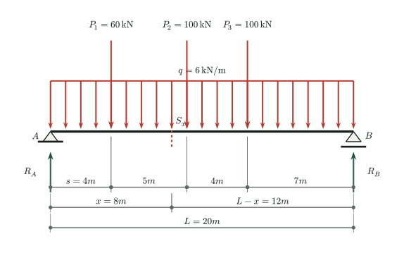
Use the generic load shown in all three figures. The lane load covers the full span independently of the vehicle position, and is added to the axle loads without an exclusion zone. These illustrative values are not taken from a design standard and do not include impact or load factors.

\[ L=20\,\mathrm m,\quad x=8\,\mathrm m,\quad s=4\,\mathrm m,\quad d_{1,2}=5\,\mathrm m,\quad d_{2,3}=4\,\mathrm m, \] \[ (P_1,P_2,P_3)=(60,100,100)\,\mathrm{kN},\quad (z_1,z_2,z_3)=(s,s+d_{1,2},s+d_{1,2}+d_{2,3}) =(4,9,13)\,\mathrm m,\quad q=6\,\mathrm{kN/m}. \]

Support reactions

Example load position: three axle loads at 4, 9, and 13 m on a 20 m beam, plus a uniform lane load of 6 kN/m over the full span. The section is at x = 8 m. Long arrows denote axle loads; shorter arrows denote the distributed load.

\[ R_A=60(0.80)+100(0.55)+100(0.35)+\frac{6(20)}2 =\boxed{198\,\mathrm{kN}}, \] \[ R_B=60(0.20)+100(0.45)+100(0.65)+\frac{6(20)}2 =\boxed{182\,\mathrm{kN}}. \]

Shear force

Same load position above the shear influence line. Dashed ordinate guides identify ηV at each axle. The shaded left area is negative (−1.60 m), and the shaded right area is positive (+3.60 m); multiply their signed sum by q, and add the three products Pi ηV(zi).

\[ (\eta_V(z_1),\eta_V(z_2),\eta_V(z_3))=(-0.20,0.55,0.35), \quad (A_V^-,A_V^+)=(-1.60,3.60)\,\mathrm m, \] \[ V_x=60(-0.20)+100(0.55)+100(0.35)+6(-1.60+3.60) =\boxed{90\,\mathrm{kN}}. \]

Bending moment

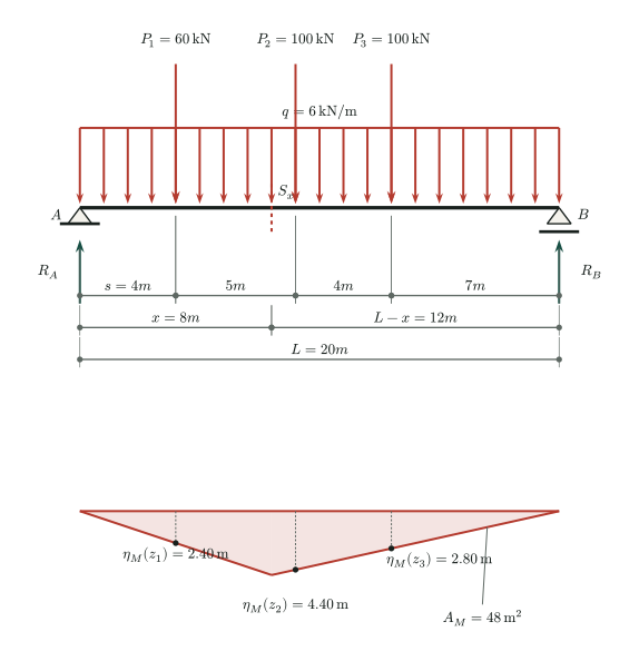
\[ (\eta_M(z_1),\eta_M(z_2),\eta_M(z_3))=(2.40,4.40,2.80)\,\mathrm m, \quad A_M=48\,\mathrm{m^2}, \] \[ M_x=60(2.40)+100(4.40)+100(2.80)+6(48) =\boxed{1152\,\mathrm{kN\,m}}. \]

Check the reactions against total vertical load, then verify the section forces directly using the left free body. Only the axle at 4 m and the first 8 m of lane load lie to the left of the cut:

\[ R_A+R_B=380=60+100+100+6(20)\quad[\mathrm{kN}], \] \[ V_x=198-60-6(8)=90\,\mathrm{kN},\qquad M_x=198(8)-60(8-4)-\frac{6(8)^2}{2}=1152\,\mathrm{kN\,m}. \]

7

Checks and limitations

The calculations above apply to an arbitrary, specified vehicle position, not necessarily the critical one. To obtain extrema at a fixed section, translate the complete axle group with its spacings preserved, including entry and exit, and evaluate every admissible distributed-load arrangement. For shear, check both sides of every axle crossing. Positive and negative shear extrema must be sought separately. Load only favorable influence-line regions when the governing load rules permit it; do not remove unfavorable loads that those rules require. Repeat for other sections to form an envelope.

This is a static, one-dimensional explanation, not a code-compliant bridge design. A design application must specify the governing standard, vehicle and lane combinations, dynamic amplification, load and combination factors, multiple-presence rules, transverse distribution to girders, and any required fatigue or serviceability checks. A qualified engineer must verify these requirements; they are not supplied by this example.

With only vertical loads in this idealized beam model, the axial force is zero. Braking, traction, horizontal actions, torsion, and local wheel-load effects require additional models.