
This note explains how to calculate the maximum and minimum shear force at a fixed section of a simply supported beam subjected to three moving concentrated loads representing a vehicle’s axles. Because the shear influence line has both a negative and a positive branch, both the largest and the smallest values must be sought during the complete passage of the vehicle.
First, the algebraic response to the passage of the complete vehicle is calculated, retaining all loads. A separate final section presents an envelope criterion that selects contributions of the same sign, without offsetting favorable contributions, when this selection is permitted by the applicable code load model.
1 Shear force for an arbitrary vehicle position
Consider a simply supported beam of span \(L\) subjected to three downward vertical concentrated loads \(P_1\), \(P_2\), and \(P_3\), which move together with positive fixed spacings \(d_{1,2}\) and \(d_{2,3}\). Let \(s\) be the vehicle reference position. The first load is located at \(s\), so that:
\[\begin{equation} z_1(s)=s,\qquad z_2(s)=s+d_{1,2},\qquad z_3(s)=s+d_{1,2}+d_{2,3}. \end{equation}\]
Define \(d_{1,3}=d_{1,2}+d_{2,3}\), giving \(z_3(s)=s+d_{1,3}\).
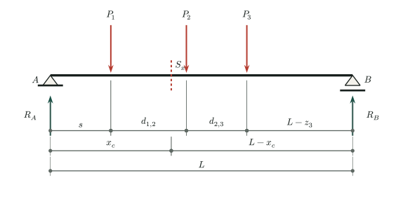
Taking shear as the left reaction minus the loads to the left of the section, the shear influence line at a fixed section \(S_x\) located at \(x_c\) is:
\[\begin{equation} V_I(z)= \begin{cases} -\dfrac{z}{L}, & 0\le z<x_c,\\[5pt] \dfrac{L-z}{L}, & x_c<z\le L,\\[5pt] 0, & z\notin[0,L]. \end{cases} \label{eq:shear-influence-line} \end{equation}\]
There is a discontinuity at \(z=x_c\). Both one-sided limits must therefore be considered:
\[\begin{equation} V_I(x_c^-)= -\dfrac{x_c}{L}, \qquad V_I(x_c^+)=\dfrac{L-x_c}{L}. \label{eq:shear-influence-jump} \end{equation}\]
The shear force for an arbitrary vehicle position is the sum of each load magnitude multiplied by the corresponding influence-line ordinate:
\[\begin{equation} V(s)=P_1V_I\bigl(z_1(s)\bigr)+P_2V_I\bigl(z_2(s)\bigr) +P_3V_I\bigl(z_3(s)\bigr). \label{eq:general-shear} \end{equation}\]
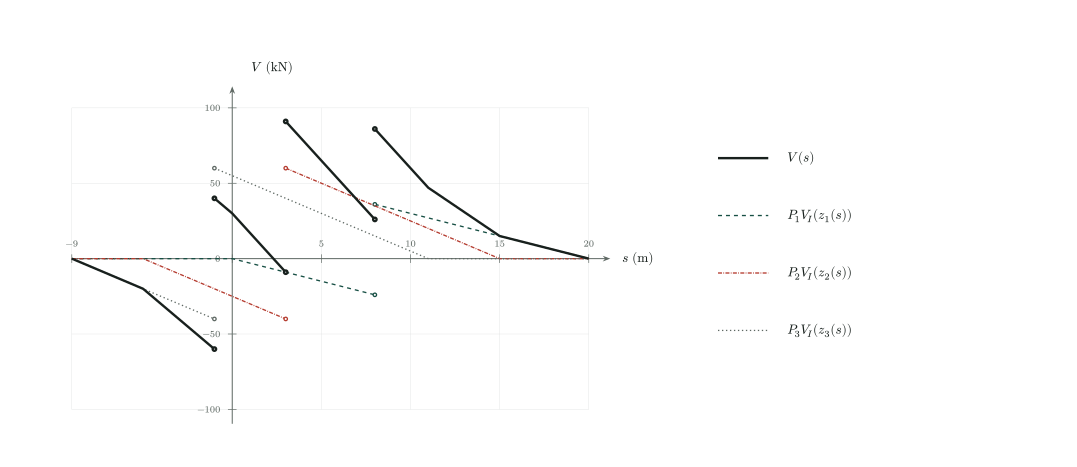
Figure 2 illustrates this sum for \(L=20\,\mathrm{m}\), \(x_c=8\,\mathrm{m}\), \(d_{1,2}=5\,\mathrm{m}\), \(d_{2,3}=4\,\mathrm{m}\), \(P_1=60\,\mathrm{kN}\), and \(P_2=P_3=100\,\mathrm{kN}\), using the same data as the numerical example below. The dashed, dash-dot, and dotted curves represent \(P_jV_I(z_j(s))\), and the solid black curve represents \(V(s)\). At the same abscissa \(s\), the three ordinates are added algebraically, retaining both positive and negative contributions. Each load produces a jump of magnitude \(P_j\) as it crosses the section, at \(s=8\), \(3\), and \(-1\,\mathrm{m}\), respectively. Open circles indicate the two one-sided limits, without connecting the jumps by inclined segments. For example, at \(s=3\,\mathrm{m}\), \(V\) jumps from \(-9\) to \(91\,\mathrm{kN}\); at \(s=-1\,\mathrm{m}\), it jumps from \(-60\) to \(40\,\mathrm{kN}\). Positive values are plotted upward and negative values downward. This is the complete-vehicle response, not the envelope excluding favorable contributions discussed in the final section.
Loads outside the span contribute nothing to shear because their influence ordinates are zero.
2 Why both the maximum and the minimum are needed
Unlike the bending-moment influence line, which is continuous within the span, the shear influence line has a jump at the fixed section. It is also negative to the left of the section and positive to the right. Different loads can therefore produce contributions with opposite signs in equation (4).
The maximum is the largest shear force reached during the movement:
\[\begin{equation} V_{\max}(x_c)=\max_s V(s), \end{equation}\]
The minimum is the smallest:
\[\begin{equation} V_{\min}(x_c)=\min_s V(s). \end{equation}\]
The largest absolute value should not be sought without first identifying its sign. Either \(V_{\max}\) or \(V_{\min}\) may govern design shear, depending on the load combination and the adopted convention.
3 Critical load positions
Away from \(x_c\), the influence line is piecewise linear. Thus, while no load crosses the section, \(V(s)\) is also piecewise linear and its extrema occur at vertices of the polygonal function. For a passing vehicle, the relevant vertices occur when a load coincides with the section.
Because there is a jump at \(x_c\), each alignment must be evaluated on both sides:
immediately before the load reaches the section, denoted by \(x_c^-\);
immediately after the load reaches the section, denoted by \(x_c^+\).
Three loads give six candidates: each load at the section, evaluated from the left and from the right. The exact position \(z_i=x_c\) need not be inserted into the sum, because the influence ordinate is discontinuous there; the one-sided limits provide the physically relevant values.
The next three figures correspond to cases a, b, and c in the bending-moment note, with all loads on the span. Each alignment is geometric: the ordinates \(V_I(x_c^-)\) and \(V_I(x_c^+)\) represent two separate evaluations, not simultaneous contributions of the same load.
3.1 Load \(P_1\) crossing the section
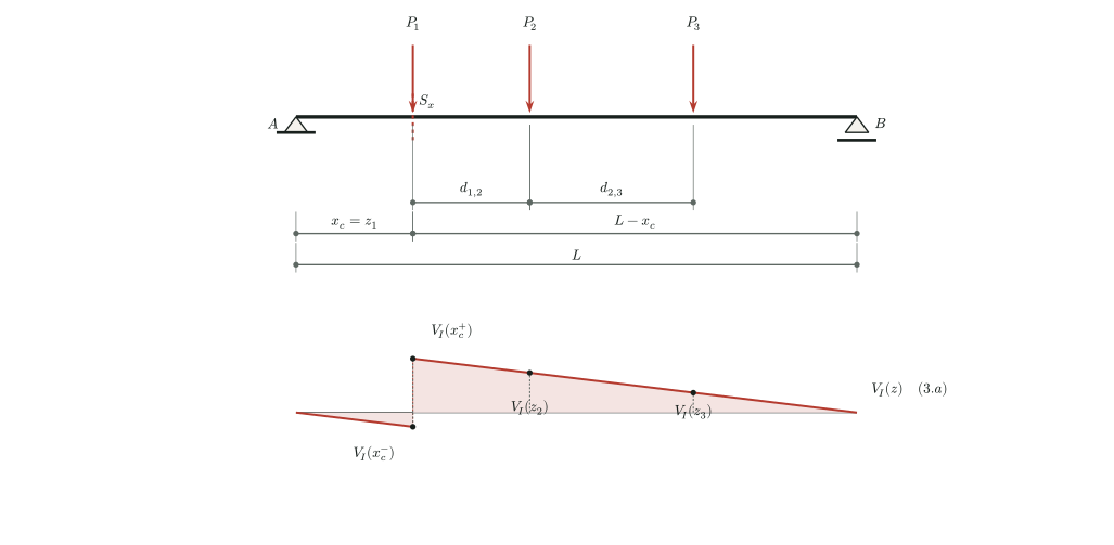
When \(P_1\) is immediately to the left of the section, the load positions are:
\[\begin{equation} z_1=x_c^-,\qquad z_2=x_c+d_{1,2},\qquad z_3=x_c+d_{1,3}. \end{equation}\]
The corresponding candidate is:
\[\begin{equation} V_{1^-}=P_1V_I(x_c^-) +P_2V_I(x_c+d_{1,2}) +P_3V_I(x_c+d_{1,3}). \end{equation}\]
When \(P_1\) is immediately to the right of the section:
\[\begin{equation} z_1=x_c^+,\qquad z_2=x_c+d_{1,2},\qquad z_3=x_c+d_{1,3}, \end{equation}\]
\[\begin{equation} V_{1^+}=P_1V_I(x_c^+) +P_2V_I(x_c+d_{1,2}) +P_3V_I(x_c+d_{1,3}). \end{equation}\]
3.2 Load \(P_2\) crossing the section
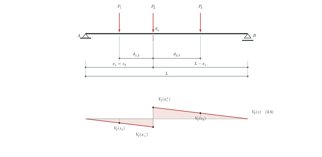
For \(P_2\) immediately to the left or right of the section, the positions are:
\[\begin{equation} z_1=x_c-d_{1,2},\qquad z_2=x_c^\mp,\qquad z_3=x_c+d_{2,3}. \end{equation}\]
The two candidates are therefore:
\[\begin{equation} \begin{aligned} V_{2^-}&=P_1V_I(x_c-d_{1,2}) +P_2V_I(x_c^-)+P_3V_I(x_c+d_{2,3}),\\ V_{2^+}&=P_1V_I(x_c-d_{1,2}) +P_2V_I(x_c^+)+P_3V_I(x_c+d_{2,3}). \end{aligned} \end{equation}\]
3.3 Load \(P_3\) crossing the section
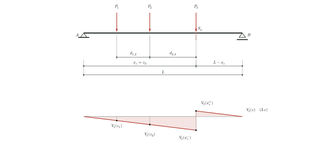
Finally, when \(P_3\) crosses the section:
\[\begin{equation} z_1=x_c-d_{1,3},\qquad z_2=x_c-d_{2,3},\qquad z_3=x_c^\mp. \end{equation}\]
The candidates are:
\[\begin{equation} \begin{aligned} V_{3^-}&=P_1V_I(x_c-d_{1,3}) +P_2V_I(x_c-d_{2,3})+P_3V_I(x_c^-),\\ V_{3^+}&=P_1V_I(x_c-d_{1,3}) +P_2V_I(x_c-d_{2,3})+P_3V_I(x_c^+). \end{aligned} \end{equation}\]
4 Critical positions with one or more loads outside the span
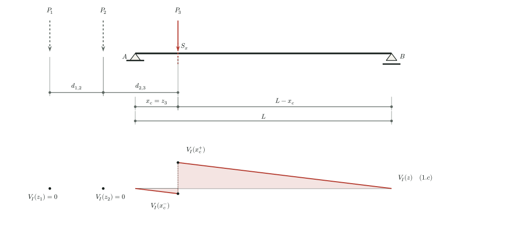
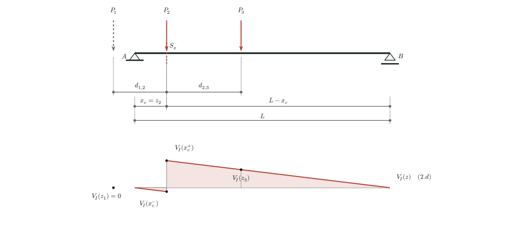
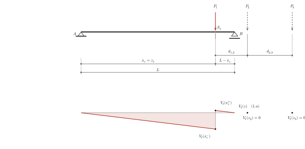
The same six candidate alignments remain valid when one or more loads are outside the beam. Their influence ordinates are zero: \(V_I(z_j)=0\) whenever \(z_j<0\) or \(z_j>L\). No additional case-specific equations are needed: retain all three load positions and evaluate the function defined in equation (2).
Figure 6 illustrates a configuration with only \(P_3\) on the span:
In figure 7, \(P_1\) is outside the span to the left, while \(P_2\) and \(P_3\) remain on the beam:
Finally, figure 8 shows a configuration with only \(P_1\) on the span:
5 General calculation of the extrema
The six preceding evaluations remain valid when one or more loads are outside the span: simply use \(V_I(z)=0\) for those loads. The general procedure is therefore to calculate:
\[\begin{equation} \mathcal{V}= \left\{V_{1^-},V_{1^+},V_{2^-},V_{2^+},V_{3^-},V_{3^+}\right\}. \end{equation}\]
The largest and smallest shear forces at the fixed section are:
\[\begin{equation} \boxed{V_{\max}(x_c)=\max\mathcal{V}}, \qquad \boxed{V_{\min}(x_c)=\min\mathcal{V}}. \label{eq:max-min-shear} \end{equation}\]
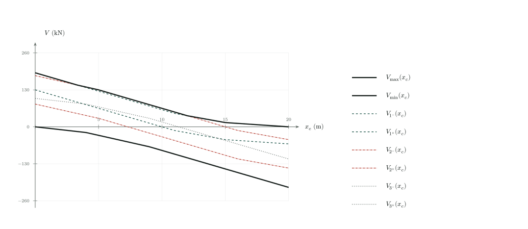
Figure 9 retains the span, loads, and spacings of the superposition figure, but varies the section position \(x_c\). For each load aligned with the section, both candidates \(V_{j^-}(x_c)\) and \(V_{j^+}(x_c)\) are shown: dashed lines for \(j=1\), dash-dot lines for \(j=2\), and dotted lines for \(j=3\). The two thick solid black curves represent \(V_{\max}(x_c)\) and \(V_{\min}(x_c)\), obtained at each abscissa by selecting the largest and smallest of the six ordinates, without adding them. Each abscissa represents an independent analysis of the complete vehicle passage at a fixed section. Unlike bending-moment candidates, shear candidates are piecewise linear in \(x_c\): load entry and exit breakpoints and intersections between candidates suffice, without dense discretization. At \(x_c=8\,\mathrm{m}\), the envelopes give \(91\,\mathrm{kN}\) and \(-60\,\mathrm{kN}\). At the graph endpoints, values represent the limits of internal sections \(x_c\to0^+\) and \(x_c\to L^-\), not a unique definition of shear exactly at a support.
The largest absolute value may be reported separately if required:
\[\begin{equation} |V|_{\max}(x_c)= \max\left\{\,|V_{\max}(x_c)|,\;|V_{\min}(x_c)|\,\right\}. \end{equation}\]
6 Numerical example
Let \(L=20\,\mathrm{m}\), \(x_c=8\,\mathrm{m}\), \(d_{1,2}=5\,\mathrm{m}\), \(d_{2,3}=4\,\mathrm{m}\), \(P_1=60\,\mathrm{kN}\), and \(P_2=P_3=100\,\mathrm{kN}\). Then:
\[\begin{equation} V_I(x_c^-)=-\frac{8}{20}=-0.4, \qquad V_I(x_c^+)=\frac{12}{20}=0.6. \end{equation}\]
Substituting the axle positions into equation (2) gives the six candidates:
\[\begin{equation} \begin{array}{c|rrrrrr} & V_{1^-} & V_{1^+} & V_{2^-} & V_{2^+} & V_{3^-} & V_{3^+}\\ \hline V\;(\mathrm{kN})& 26&86&-9&91&-60&40 \end{array} \end{equation}\]
Thus:
\[\begin{equation} \boxed{V_{\max}=91\,\mathrm{kN}}, \qquad \boxed{V_{\min}=-60\,\mathrm{kN}}. \end{equation}\]
The largest absolute value is \(|V|_{\max}=91\,\mathrm{kN}\), corresponding to the algebraic maximum. This example shows why both extrema must be evaluated when the influence line has branches with opposite signs: the governing case can change with load magnitudes and spacings.
At support sections, the analysis must follow the shear convention and the side of the section considered. For an internal section \(0<x_c<L\), the above procedure directly accounts for the jump and for loads outside the span.
7 Envelope with contributions of the same sign
7.1 Distinguishing vehicle passage from the envelope criterion
So far, \(V(s)\) is the complete-vehicle response. A load on the negative branch reduces the response produced by loads on the positive branch, and vice versa. This offset is correct for the physical response of that vehicle at that position, but it does not represent the envelope criterion excluding favorable contributions used in this section.
For bridge envelopes, when the applicable code load model requires the selection of unfavorable contributions, only contributions of the same sign are considered: positive for the maximum and negative for the minimum. Two loads on one side of the section may therefore produce a more critical envelope effect than those two loads combined with a third load on the opposite-sign branch.
This selection must comply with the applicable code, its edition, and its definitions of actions or load groups. It is not a general authorization to remove axles from a real vehicle or to select individual contributions from any permanent action. The following expressions formalize the requested criterion for the three moving loads, assuming their favorable contributions may be disregarded. Code factors and combinations must be applied as appropriate to the design case.
7.2 Separating positive and negative contributions
For \(P_i>0\), define two functions from the signed influence-line ordinates:
\[\begin{equation} V_I^{(+)}(z)=\max\{V_I(z),0\}, \qquad V_I^{(-)}(z)=\min\{V_I(z),0\}. \end{equation}\]
The parenthesized superscript denotes selection by sign, not the side of the jump. For example:
\[\begin{equation} \begin{aligned} V_I^{(+)}(x_c^-)&=0, & V_I^{(+)}(x_c^+)&=\frac{L-x_c}{L},\\ V_I^{(-)}(x_c^-)&=-\frac{x_c}{L}, & V_I^{(-)}(x_c^+)&=0. \end{aligned} \end{equation}\]
For each vehicle position, calculate separately:
\[\begin{equation} \begin{aligned} V^{(+)}(s)&=\sum_{i=1}^{3}P_iV_I^{(+)}\bigl(z_i(s)\bigr),\\ V^{(-)}(s)&=\sum_{i=1}^{3}P_iV_I^{(-)}\bigl(z_i(s)\bigr). \end{aligned} \label{eq:shear-sign-selection} \end{equation}\]
In the first sum, a load on the negative branch contributes nothing. In the second, a load on the positive branch contributes nothing. Loads outside the span contribute zero to both sums. The original spacings are preserved: selection excludes favorable contributions but does not bring the remaining axles closer together or reposition them independently.
The complete-vehicle response satisfies \(V(s)=V^{(+)}(s)+V^{(-)}(s)\). However, for this envelope, these two contributions must not be added before seeking the extrema.
7.3 Critical positions and envelope extrema
With \(a_1=0\), \(a_2=d_{1,2}\), and \(a_3=d_{1,3}\), the preceding alignments are \(s_k=x_c-a_k\), for \(k=1,2,3\). At each alignment, evaluate both one-sided limits of the entire sum:
\[\begin{equation} C_{k,\pm}^{(+)}=\lim_{s\to s_k^\pm}V^{(+)}(s), \qquad C_{k,\pm}^{(-)}=\lim_{s\to s_k^\pm}V^{(-)}(s). \end{equation}\]
The envelope extrema without offsetting favorable contributions are:
\[\begin{equation} \boxed{V_{\max,\mathrm{env}}(x_c)= \max\left(\{0\}\cup\{C_{k,\pm}^{(+)}:k=1,2,3\}\right)}, \end{equation}\]
\[\begin{equation} \boxed{V_{\min,\mathrm{env}}(x_c)= \min\left(\{0\}\cup\{C_{k,\pm}^{(-)}:k=1,2,3\}\right)}. \label{eq:shear-envelope-extremes} \end{equation}\]
Zero includes the unloaded configuration and ensures a nonnegative maximum and a nonpositive minimum. The candidate search remains based on the three loads crossing the section, using both one-sided limits and zero ordinates for loads outside the span.
In the figures for cases a, b, and c, the two sides of the jump make this selection explicit. For example, in case b, with \(P_2\) immediately to the right of the section, \(P_2\) and \(P_3\) may contribute to the maximum, but the negative contribution of \(P_1\) is disregarded. With \(P_2\) immediately to the left, \(P_1\) and \(P_2\) may contribute to the minimum, without the positive offset from \(P_3\). The same rule applies to the figures with loads outside the span.
7.4 Comparison using the numerical example
Using the same data and alignments as in the preceding example gives:
\[\begin{equation} \begin{array}{c|rrrrrr} & 1^- & 1^+ & 2^- & 2^+ & 3^- & 3^+\\ \hline V^{(+)}\;(\mathrm{kN}) & 50 & 86 & 40 & 100 & 0 & 60\\ V^{(-)}\;(\mathrm{kN}) & -24 & 0 & -49 & -9 & -60 & -20\\ V\;(\mathrm{kN}) & 26 & 86 & -9 & 91 & -60 & 40 \end{array} \end{equation}\]
At alignment \(2^+\), the positions are \(z_1=3\,\mathrm{m}\), \(z_2=8^+\,\mathrm{m}\), and \(z_3=12\,\mathrm{m}\). The contributions are \(-9\,\mathrm{kN}\), \(60\,\mathrm{kN}\), and \(40\,\mathrm{kN}\). The complete-vehicle response is \(91\,\mathrm{kN}\), but the envelope maximum without offset is \(60+40=100\,\mathrm{kN}\) because the favorable contribution \(-9\,\mathrm{kN}\) is excluded.
Therefore:
\[\begin{equation} \boxed{V_{\max,\mathrm{env}}=100\,\mathrm{kN}}, \qquad \boxed{V_{\min,\mathrm{env}}=-60\,\mathrm{kN}}. \end{equation}\]
In this example, the minimum is unchanged because its critical alignment already has no positive contribution. In general:
\[\begin{equation} V_{\max,\mathrm{env}}\ge V_{\max}, \qquad V_{\min,\mathrm{env}}\le V_{\min}. \end{equation}\]
These results distinguish the algebraic complete-vehicle response from the envelope obtained by selecting same-sign contributions, preventing favorable contributions from reducing the extrema when the adopted loading criterion does not permit that reduction.